A last section demonstrates the use of the barrier synchronization elements that are part of FSF.
disclaimer
The code appearing in this guide was developed by the author, and is part of open source libraries, modules and examples released under the GNU Lesser General Public License. They are available for download on the MFSM web site. This code is provided here in the hope that it will be useful, but without any warranty; without even the implied warranty of merchantability or fitness for a particular purpose. Complete license information is provided in the downloadable packages.
sai in a nutshell
The Software Architecture for Immersipresence (SAI) framework (Francois, 2010) offers a unifying approach to the distributed implementation of algorithms and their easy integration into complex systems that exhibit desirable qualities such as efficiency, scalability, extensibility, reusability and interoperability. SAI provides a general formalism for the design, analysis and implementation of complex software systems of asynchronous interacting processing components. The SAI model builds on three pilars: (1) explicit account of time both in data and processing models; (2) distinction between persistent and volatile data; (3) asynchronous concurrency.
SAI specifies an architectural style (Francois, 2004) that combines an extensible data model and a hybrid (shared memory and message-passing) distributed asynchronous concurrent processing model. Figure 1 presents an overview of SAI defining elements in their standard notation.
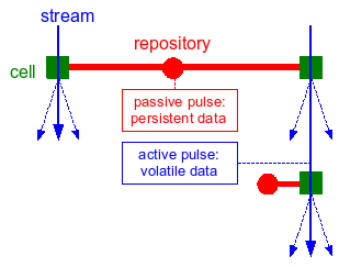
Figure 1: Overview of SAI elements. Cells are represented as
squares, repositories as circles. Repository-cell connections are drawn as fat
lines, while cell-cell connections are drawn as thin arrows crossing
over the cells. When color is available, cells are colored in green
(reserved for processing); repositories, repository-cell connections, passive
pulses are in colored in red (persistent information); streams and
active pulses are colored in blue (volatile information).
In SAI, all data is encapsulated in pulses. A pulse is the carrier for all the synchronous data corresponding to a given time stamp. Information in a pulse is organized as a mono-rooted composition hierarchy of node instances. The nodes constitute an extensible set of atomic data units that implement or encapsulate specific data structures. Pulses holding volatile data flow down streams defined by connections between processing centers called cells, in a message passing fashion. They trigger computations, and are thus called active pulses. In contrast, pulses holding persistent information are held in repositories called repositories, where the processing centers can access them in a concurrent shared memory access fashion. Processing in a cell may result in the augmentation of the active pulse (input data), augmentation and/or update of the passive pulse (process parameters). The processing of active pulses is carried in parallel, as they are received by the cell. Data binding is performed dynamically in an operation called {em filtering}. Active and passive filters qualitatively specify, for each cell, the target data in respective pulses. This hybrid model combining message passing and shared repository communication, combined with a unified data model, constitutes a universal processing framework.
A particular system architecture is specified at the conceptual level by a set of repository and cell instances, and their inter-connections. The logical level specification of a design describes, for each cell, its active and passive filters and its output structure, and for each repository, the structure of its passive pulse.
notations
The graphical notation introduced above is sufficient for specifying systems at the conceptual level--a set of repository and cell instances, and their inter-connections. The specialized cells may be accompanied by a description of the task they implement. Repository and cell instances may be given names for easy reference. In some cases, important data nodes and outputs may be specified schematically to emphasize some design aspects.
Logical level specifications require additional notation conventions to represent nodes (and pulses) and filters.
Specialized node types are identified by their type name (string). Node instances are identified by their (instance) name. The notation adopted to represent node instances and hierarchies of node instances makes use of nested parentheses, e.g.: (NODE_TYPE_ID ``Node name'' (...) ... ). This notation will be used to specify a cell's output, and for logical specification of active and passive pulses.
The notation adopted for specifying filters and hierarchies of filters is nested square brackets. Each filter specifies a node type, a node instance name or name pattern (with wildcard characters), an optional handle name, and an optional list of subfilters, e.g.: [NODE_TYPE_ID ``Node name'' handle_id [...] ... ]. Optional filters are indicated by a star, e.g.: [NODE_TYPE_ID ``Node name'' handle_id]*.
The table below summarizes the notations for logical level cell definition using the nested square brackets and nested parentheses notations introduced above for filters and nodes respectively. By convention, in the cell output specification, (x) represents the pulse's root, (.) represents the node corresponding to the root of the active filter, and (..) represents its parent node.
| ClassName (ParentClass) | CELL_TYPE_ID |
| Active filter | [NODE_TYPE_ID "Node name" [...] ... ] |
| Passive filter | [NODE_TYPE_ID "Node name" [...] ... ] |
| Output | (NODE_TYPE_ID "default output base name--more if needed" (...) ... ) |
| Short description of process behavior | |
a first example
In this section, a simple example console application, called
example1, illustrates all the steps from design to implementation.
The code for the examples in this guide are part of the MFSM
distribution, and can be downloaded from
the MFSM project
page on SourceForge.net.
Suppose the goal of the program is to generate a stream at a given frame rate, and display the time stamp of each pulse in seconds and in h/m/s formats. Note that in MFSM version 0.8 and higher, the time stamp is the number of nanoseconds elapsed since the Epoch (00:00:00 UTC, January 1, 1970) on Mac OS X and Linux platforms, and the number of nanoseconds elapsed since the system was last booted on Win32 platforms.
Fsf defines a fsf::Time type, typedefed
to double since version 1.0.
FSF contains a fundamental cell used to generate empty pulses at a given frame rate: the Pulsar. Its specifications are as follows:
| fsf::CPulsar (fsf::CCell) | FSF_PULSAR |
| Active filter | (no input) |
| Passive filter | [FSF_FLOAT64_NODE "Pulse delay"] |
| Output | (FSF_ACTIVE_PULSE "Root") |
| Places an empty pulse on the active stream at specified time interval | |
A pulsar does not have any input. One parameter, of integral type, specifies the time delay between two consecutive output pulses.
In this section, a cell capable of looking up the time stamp of each incoming active pulse and printing it to the console in a given format, is assumed to be available. The actual implementation of this cell is addressed in the next section which addresses custom cells. The cell specifications are as follows:
| ex1::CPrintTime (fsf::CCell) | PRINT_TIME |
| Active filter | [FSF_ACTIVE_PULSE "Root"] |
| Passive filter | [FSF_PASSIVE_PULSE "Root"] |
| Output | (no output) |
| Writes to cout the timestamp of incoming active pulses in s, and in h/m/s | |
It is straightforward to implement our simple application from from
one instance of CPulsar and one instance of
CPrintTime. Figure 2 shows the
conceptual system graph.
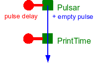
Figure 2: Conceptual system graph for example1
Two functional units can be identified:
- the pulsing unit, comprising a pulsar cell and its associated repository, and
- the display unit, comprising the PrintTime cell and its associated repository.
The following subsections explain in detail how to code the simple application in C++: setup the system, build and run the application graph, clean-up the objects allocated.
setting-up the system
The unique instance of the system class is automatically created when first needed (Singleton pattern). First and foremost, the nodes and cells defined in each module used must be registered with the system. As a result, although FSF is highly multi-threaded, the unique instance will be allocated before multi-threading kicks in, and thus a double lock mechanism is probably not needed in the implementation of the CSystem class.
Factories can be registered in any order. They are not necessary
for pre-coded application graphs, although they are used by the system
functions that instantiate cells and nodes based on their type ID
strings. Factories are necessary for dynamic, run-time application
graph building and/or modification, which is out of the scope of this
introduction. Each module is required to declare and implement a
function called registerFactories for registering
factories in the system for all nodes and cells implemented in the
module.
    // register system factories
    fsf::registerFactories();

    // register ex1 factories
    ex1::registerFactories();
building the graph
The CSystem and CCell classes provide
high-level functions to instantiate repositories and cells, instantiate
nodes and place them in repository pulses, connect cells to other cells
and to repositories.
The code for building an application graph instantiates and connects all the elements of the conceptual graph. In this simple example, the graph can be divided into two functional subgraphs: the pulsing unit, built around an instance of Pulsar, and the display unit built around an instance of PrintTime. Each functional subgraph in this case corresponds to one repository and one cell (minimal computing units).
Each minimal unit, consisting of one cell and one repository whose pulse contains the cell's parameters, can be coded following these steps:
- Instantiate the repository.
- Instantiate the parameter node(s). Each node is placed in the repository's passive pulse hierarchy. Optional steps for each node include setting its name and data member initial values.
- Instantiate the cell. Optional steps include setting the output base name, the active and passive filters. The cell is then connected to its repository, and to the cell directly upstream on the active stream, if any.
These principles can be used as general guidelines and adapted to
code any graph. The following code builds the graph for example1,
first the pulsing unit, then the display unit. Successful
instantiation of all graph elements is checked, as failure to register
the appropriate factories will result in the failure to instantiate a
given cell or node.
    // build graph
    bool bSuccess=true;

    ////////////
    // Pulsar //
    ////////////

    // create the repository
    fsf::CRepository *pPRepository=new fsf::CRepository;
    bSuccess &= (pPRepository!=NULL);

    // parameter nodes
    fsf::Float64Node *pPulseRate=static_cast<fsf::Float64Node*>(
	fsf::CSystem::createNode(std::string("FSF_FLOAT64_NODE"),pPRepository->getPulse()));
    bSuccess &= (pPulseRate!=NULL);
    if(bSuccess){
	// set name
	pPulseRate->setName(std::string("Pulse delay"));
	// set parameter values
	fsf::Time tPulseDelay=static_cast<fsf::Time>(1000000000.0f/fPulseRate);
	pPulseRate->setData(tPulseDelay);
    }

    // cell
    fsf::CCell *pPcell=fsf::CSystem::createCell(std::string("FSF_PULSAR"));
    bSuccess &= (pPcell!=NULL);
    if(bSuccess){
	// connect with repository
	pPcell->connectRepository(pPRepository);
    }

    //////////////////////
    // Print time stamp //
    //////////////////////

    // create the repository
    fsf::CRepository *pIRepository=new fsf::CRepository;
    bSuccess &= (pIRepository!=NULL);

    // cell
    fsf::CCell *pPrintTime=fsf::CSystem::createCell(std::string("PRINT_TIME"));
    bSuccess &= (pPrintTime!=NULL);
    if(bSuccess){
	// connect with repository
	pPrintTime->connectRepository(pIRepository);
	// connect with Pcell
        pPrintTime->connectUpstreamCell(pPcell);
    }

    // Check everything went OK...

    if(bSuccess==false){
	cout << "Some elements in the graph could not be instantiated..." << endl;
	return (-1);
    }
running the graph
Once the graph is completed, the cells must be activated. The Pulsar instance is the origin of the active stream and starts generating empty pulses as soon as it is activated. The PrintTime instance, once activated, will process incoming pulses concurrently, asynchronously. The cells can be started in any order.
    // Run
    pPrintTime->on();
    pPcell->on();
cleaning-up
Although this aspect is not evident in this simple example, cells can be turned on and off at any time, elements (repositories and cells) can be connected and disconnected at any time, new ones can be created and existing ones destroyed at any time.
The following code stops the cells, disconnects and destroys the different elements instantiated when building the graph, and finally destroys the unique system instance.
    // Stop the cells
    cout << "Stopping the cells..." << endl;
    pPcell->off();
    pPrintTime->off();

    // Clean up
    cout << "Cleaning-up..." << endl;

    pPcell->disconnectRepository();
    pPcell->disconnectStream();
    delete pPcell;
    delete pPRepository;

    pPrintTime->disconnectRepository();
    pPrintTime->disconnectStream();
    delete pPrintTime;
    delete pIRepository;

    // Delete unique system instance
    fsf::CSystem::deleteInstance();
running the program
The example implementation allows the user to specify the pulse rate on the command line (the default rate is 30 Hz). Below is a sample output from the program.
>example1 -f 30
MFSM Example1
Alexandre R.J. Francois
(C) 2010
Requested pulse rate: 30 Hz
Pulse: 1.28658e+09 s = 357383 h 38 min 39 s
Pulse: 1.28658e+09 s = 357383 h 38 min 39 s
Pulse: 1.28658e+09 s = 357383 h 38 min 39 s
Pulse: 1.28658e+09 s = 357383 h 38 min 39 s
Pulse: 1.28658e+09 s = 357383 h 38 min 39 s
Pulse: 1.28658e+09 s = 357383 h 38 min 39 s
Pulse: 1.28658e+09 s = 357383 h 38 min 39 s
Pulse: 1.28658e+09 s = 357383 h 38 min 39 s
Pulse: 1.28658e+09 s = 357383 h 38 min 40 s
Pulse: 1.28658e+09 s = 357383 h 38 min 40 s
Pulse: 1.28658e+09 s = 357383 h 38 min 40 s
Pulse: 1.28658e+09 s = 357383 h 38 min 40 s
Pulse: 1.28658e+09 s = 357383 h 38 min 40 s

Stopping the cells...
Cleaning-up...
Quitting program.
custom cells
If one of the goals of MFSM is to facilitate rapid development of
applications from existing modules, one of its main strenghts is to
enable easy development of custom elements that will interoperate
seamlessly with existing or third party components. The example
developed in the previous section, example1, uses the
PrintTime cell to look up the time stamp of each incoming active pulse
and print it to the console in a given format. This section details
how to describe and implement such custom cells.
time stamp display
Any cell class must be derived from the base cell class
(CCell). It is characterized by an identification string
(used for to link it to its factory). A complete description includes
the active and passive filters, the process output, a list of data
members and member functions with a short description.
A custom cell must implement the default constructor, and overload a number of virtual functions which characterize the cell:
getTypeID(const): returns the factory mapping key.process: theprocessfunction is the only one requiring significant coding, as it is the place to specialize the behavior of the cell.
When the function is called, the binding has already succeeded and it is executed in a separate thread.
For the cell to be useful, the process function must be described carefully. In particular, the way the input is processed and any output generated should be carefully documented.
Custom elements for example1 are placed in
the ex1 namespace. The logical specifications of the
cell CPrintTime used in example1 are as
follows:
| ex1::CPrintTime (fsf::CCell) | PRINT_TIME |
| Active filter | [FSF_ACTIVE_PULSE "Root"] |
| Passive filter | [FSF_PASSIVE_PULSE "Root"] |
| Output | (no output) |
| Writes to cout the timestamp of incoming active pulses in s, and in h/m/s | |
See
the Doxygen-generated reference
guide for
a description
of CPrintTime.
The following code is the definition of
class CPrintTime:
    /// A custom cell that writes to cout the timestamp
    /// of incoming active pulses in s, and in h/m/s
    class CPrintTime : public fsf::CCell {
    public:
	/// Default constructor
	CPrintTime();

	/// Gets this cells' factory mapping key
	virtual void getTypeID(std::string &str) const { str.assign("PRINT_TIME"); }

	/// Custom processing function: writes to cout
	/// the timestamp of incoming active pulses in s, and in h/m/s
	virtual void process(fsf::CPassiveHandle *pPassiveHandle, fsf::CActiveHandle *pActiveHandle, fsf::CActivePulse *pActivePulse);
    };
The default constructor sets the default output name base, and instantiates both passive and active filters from the corresponding template classes.
    CPrintTime::CPrintTime() : CCell() {
	// default output name
	setOutputName("Doesn't matter...");
	// set the filters
	setActiveFilter(new fsf::CActiveFilter<fsf::CActivePulse>(std::string("Root")));
	setPassiveFilter(new fsf::CPassiveFilter<fsf::CPassivePulse>(std::string("Root")));
    }
When the process function is executed, filtering of
passive and active streams has succeeded. The active and passive
handles are thus bound to the nodes satisfying the filters. When the
filters are complex (hierarchies of filters), the passive and active
handles point to their respective roots. For this very simple cell,
no output is generated. The code for CPrintTime::process
is as follows:
    void CPrintTime::process(fsf::CPassiveHandle *pPassiveHandle, fsf::CActiveHandle *pActiveHandle, fsf::CActivePulse *pActivePulse){
	fsf::CNode *pNode=static_cast<fsf::CNode*>(pActiveHandle->getNode());
	double tsec=pNode->getTime()/1000000000.0;

	double h,m,s;
	double rh = modf(tsec/3600.0,&h)*3600.0;
	double rm = modf(rh/60.0,&m)*60.0;
	modf(rm,&s);
	cout << "Pulse: " << tsec << " s = " << h << " h " << m << " min " << s << " s " << endl;
    }
Factory registration
Any module must define a registerFactories function that
registers its node and cell factories with the system. Following is the code
for the registerFactories function that registers the factory for
the CPrintTime class.
    /// Factory registration.
    /// Function to call to instantiate and register factories for all
    /// nodes and cells defined in this module
    void registerFactories(){
	using namespace fsf;

	std::string strAlex("Alexandre R.J. Francois");

	////////////////////////////////////////////////
	// Node factories
	////////////////////////////////////////////////////////

	////////////////////////////////////////////////
	// Cell factories
	////////////////////////////////////////////////////////

	CSystem::getInstance()->registerCellFactory(
	    std::string("PRINT_TIME"),
	    new CCellFactory<CPrintTime>(std::string("Print time stamp"),strAlex));
    }
pulse frequency display
Here is a slightly more complex example,
called example2. The goal is now to display not the pulse
time stamp, but the pulse frequency. This requires to compute the time
delay between two consecutive pulses. Some data must therefore be
shared between the threads processing each pulse: the time stamp of
the last pulse processed is saved in a node on the passive pulse. Each
time the process function is called, the last time stamp value is
retrived from the node, and the node value is updated with the time
stamp of the pulse being processed. The difference between the two
time stamps is then computed and formatted to be output to the
console. The corresponding cell will be
called CPrintInterval.
Custom elements for example2 are placed in
the ex2 namespace.
Figure 3 shows the conceptual level system graph.
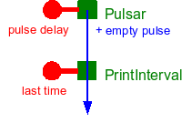
Figure 3: Conceptual system graph for example2
The logical specifications for CPrintInterval are as follows:
| ex2::CPrintInterval (fsf::CCell) | PRINT_INTERVAL |
| Active filter | [FSF_ACTIVE_PULSE "Root"] |
| Passive filter | [FSF_FLOAT64_NODE "Last time"] |
| Output | (no output) |
| Writes to cout the difference between two consecutive incoming active pulses, in s | |
See
the Doxygen-generated reference
guide for
a description
of CPrintInterval.
The definition of CPrintInterval is almost identical
to that of CPrintTime. The only differences are to the
passive filter in the constructor, and to the process
function.
The code for CPrintInterval's constructor is as follows:
    /// A custom cell that writes to cout the difference
    /// between two consecutive incoming active pulses, in s and Hz
    class CPrintInterval : public fsf::CCell {
    public:
	/// Default constructor
	CPrintInterval();

	/// Gets this cell's actory mapping key
	virtual void getTypeID(std::string &str) const { str.assign("PRINT_INTERVAL"); }

	/// Custom processing function: writes to cout
	/// the difference between the time stamp of the incoming active puse, and the last time stamp recorded.
	virtual void process(fsf::CPassiveHandle *pPassiveHandle, fsf::CActiveHandle *pActiveHandle, fsf::CActivePulse *pActivePulse);
    };
}
Note the change in the passive filter: in order to compute a delay, the
process function must access and update the value of the
time stamp of the last pulse handled.
The code for function CPrintInterval::process is as follows:
    void CPrintInterval::process(fsf::CPassiveHandle *pPassiveHandle, fsf::CActiveHandle *pActiveHandle, fsf::CActivePulse *pActivePulse){
	fsf::Float64Node *pLastTime=static_cast<fsf::Float64Node*>(pPassiveHandle->getNode());
	fsf::CNode *pNode=static_cast<fsf::CNode*>(pActiveHandle->getNode());

	if(doReset()){
	    pLastTime->setData(pNode->getTime());
	    setReset(false);
	}
	else{
	    // get last time value
	    fsf::Time tLastTime=static_cast<fsf::Time>(pLastTime->getData());
	    // update last time recorded with current pulse time stamp value
	    pLastTime->setData(pNode->getTime());

	    // compute and print time difference and corresponding frequency
	    fsf::Time dtms=(pNode->getTime()-tLastTime)/1000000.0;
	    cout << "Pulse interval: " << dtms << " ms <=> "
		 << 1000.0/dtms << " Hz"
		 << endl;
	}
    }
}
The code for building the application graph
for example2 is very similar to that
of example1. The only difference is in the output
subgraph: the node storing the "last time stamp" value must be
instantiated and placed on the passive pulse held
by pIRepository. Of course, the cell to be instantiated
now is of type PRINT_INTERVAL. The corresponding code is
as follows:
    ////////////////////
    // Print interval //
    ////////////////////

    // create the repository
    fsf::CRepository *pIRepository=new fsf::CRepository;
    bSuccess &= (pIRepository!=NULL);

    // last time stamp
    fsf::Float64Node *pLastTime=static_cast<fsf::Float64Node*>(fsf::CSystem::createNode(std::string("FSF_FLOAT64_NODE"),pIRepository->getPulse()));
    bSuccess &= (pLastTime!=NULL);
    if(bSuccess){
	// set name
	pLastTime->setName(std::string("Last time"));
    }

    // cell
    fsf::CCell *pPrintInterval=fsf::CSystem::createCell(std::string("PRINT_INTERVAL"));
    bSuccess &= (pPrintInterval!=NULL);
    if(bSuccess){
	// connect with repository
	pPrintInterval->connectRepository(pIRepository);
	// connect with Pcell
	pPrintInterval->connectUpstreamCell(pPcell);
    }
The example implementation allows the user to specify the pulse rate on the command line (the default rate is 30 Hz). Below is a sample output from the program.
>example2 -f 30
MFSM Example2
Alexandre R.J. Francois
(C) 2010
Requested pulse rate: 30 Hz
Starting cells...
Pulse interval: 33.5191 ms <=> 29.8337 Hz
Pulse interval: 33.5849 ms <=> 29.7753 Hz
Pulse interval: 33.6251 ms <=> 29.7397 Hz
Pulse interval: 33.5519 ms <=> 29.8046 Hz
Pulse interval: 33.62 ms <=> 29.7442 Hz
Pulse interval: 33.5852 ms <=> 29.7751 Hz
Pulse interval: 33.579 ms <=> 29.7805 Hz
Pulse interval: 33.557 ms <=> 29.8 Hz
Pulse interval: 33.5908 ms <=> 29.7701 Hz
Pulse interval: 33.5142 ms <=> 29.8381 Hz
Pulse interval: 33.5698 ms <=> 29.7887 Hz
Pulse interval: 33.577 ms <=> 29.7823 Hz

Stopping the cells...
Cleaning-up...
Quitting program.
custom nodes
The definition and implementation of custom nodes is illustrated
in example2b. Based on example2, this
example implements a feedback system that adjusts the pulsar rate so
that the measured time interval between pulses on the stream is as
close as possible to a target time interval.
Figure 4 shows the conceptual level system graph.
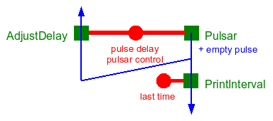
Figure 4: Conceptual system graph for example2b
The system instantiates the ex2b::CPrintInterval cell
(identical to ex2::CPrintInterval), and a new cell type
named ex2b::CAdjustDelay.
Custom elements for example2b are placed in
the ex2b namespace.
The logical specifications for CAdjustDelay are as follows:
| ex2b::CAdjustDelay (fsf::CCell) | ADJUST_DELAY |
| Active filter | [FSF_ACTIVE_PULSE "Root"] |
| Passive filter | [PULSAR_CONTROL "Pulsar control"] |
| Output | (no output) |
| Adjusts the pulsar delay based on the measured time interval between consecutive active pulses in order to bring the measured interval as close as possible to a target time interval | |
Note the passive filter: in order to compute a new pulse delay, the
process function must access and update the last time
stamp recorded and the target time interval. This information is
stored in a custom type node CPulsarControl.
See
the Doxygen-generated reference
guide for
a description
of CAdjustDelay.
Any node type specialization must be derived from the base node
fsf::CNode or a derived node. A node type is characterized by an
identification string (used to link it to its factory). A complete node type
description includes a list of data members and member functions, and a short
description of its semantics.
The CPulsarControl node class is derived directly from
the base CNode class defined in the FSF
library. CPulsarControl has two member variables of
time fsf::Time that store the target time interval and
the last recorded time stamp.
    class CPulsarControl : public fsf::CNode {
    private:
	fsf::Time m_tTargetInterval; ///< The target time interval
	fsf::Time m_tLastTime; ///< The last time stamp recorded
Any custom node class must implement a number of constructors: the default constructor, all the constructors defined in the the base node class (these must define default values for the local data members), additional constructors for specifying local data members initial values, and the copy constructor. When necessary, the virtual destructor must also be overridden.
    public:
	/// Default constructor
	CPulsarControl() : CNode() {}
	/// 2-parameter constructor: parent and timestamp
	CPulsarControl(CNode *pParent, Time tTime=0)
	    : CNode(pParent,tTime) {}
	/// 3-parameter constructor: name, parent and timestamp
	CPulsarControl(const std::string &strName,CNode *pParent=NULL, Time tTime=0)
	    : CNode(strName,pParent,tTime) {}
	/// Copy constructor
	CPulsarControl(const CPulsarControl& rhs);
No destructor override is needed here, since the destructor for the character buffer parent class takes care of deallocating the buffer if needed.
A custom node class must also override the clone
function, which returns a pointer to a copy of the node. This virtual
function is necessary for run-time polymorphism. It makes it possible
to create an instance of a specialized node class without knowing the
specific type at compile time.
	/// Cloning: necessary for run-time polymorphism
	virtual CNode *clone() const { return new CPulsarControl(*this); }
A custom node class must also override the assignment operator
	/// Assignment operator
	CPulsarControl& operator=(const CPulsarControl& rhs);
A custom node class must also override
the getTypeID const function, which returns
the node's factory mapping key.
	/// Returns this node type's factory mapping key
	virtual void getTypeID(std::string &str) const { str.assign("PULSAR_CONTROL"); }
A set of member functions provides basic access to local data
members (set and get operations), and the stepControl
function encpasupates the operations involved in the computation of a
new time interval based on the measured time stamp, the last recorded
time stamp and the target interval.
        /// Manipulators

	/// Sets this node's target interval attribute value
	void setTargetInterval(fsf::Time t) { m_tTargetInterval=t; }
	/// Sets this node's last recorded time stamp attribute value
	void setLastTime(fsf::Time t) { m_tLastTime=t; }

	/// Computes a pulsar delay value based on the target
	/// interval, the last recorded time stamp and the measured
	/// time stamp argument.  Updates last recorded time stamp.
	inline fsf::Time stepControl(double dMeasuredTime);


	/// Accessors

	/// Gets this node's target interval attribute value
	fsf::Time getTargetInterval() const { return m_tTargetInterval; }
	/// Gets this node's last recorded time stamp attribute value
	fsf::Time getLastTime() const { return m_tLastTime; }
Any module must define a registerFactories function
that registers its custom node and cell factories with the
system. Following is the code for
the ex2b::registerFactories function, which registers
factories for the custom node type ex2b::CPulsarControl,
and for the two custom cell types ex2b::CAdjustDelay
and ex2b::CPrintInterval.
    /// Factory registration.
    /// Function to call to instantiate and register factories for all
    /// nodes and cells defined in this module
    void registerFactories(){
	using namespace fsf;

	std::string strAlex("Alexandre R.J. Francois");

	////////////////////////////////////////////////
	// Node factories
	////////////////////////////////////////////////////////

	CSystem::getInstance()->registerNodeFactory(
	    std::string("PULSAR_CONTROL"),
	    new CNodeFactory<CPulsarControl>(std::string("Pulsar control node"),strAlex));

	////////////////////////////////////////////////
	// Cell factories
	////////////////////////////////////////////////////////

	CSystem::getInstance()->registerCellFactory(
	    std::string("ADJUST_DELAY"),
	    new CCellFactory<CAdjustDelay>(std::string("Adjust delay cell"),strAlex));
	CSystem::getInstance()->registerCellFactory(
	    std::string("PRINT_INTERVAL"),
	    new CCellFactory<CPrintInterval>(std::string("Print time interval"),strAlex));
    }
See
the Doxygen-generated reference
guide for
a detailed description
of CPulsarControl.
The example implementation allows the user to specify the target pulse rate on the command line (the default rate is 30 Hz). Below is a sample output from the program.
>example2b -f 30
FSM Example 2b
Alexandre R.J. Francois
(C) 2010
Requested pulse rate: 30 Hz
Starting cells...
Pulse interval: 33.514 ms <=> 29.8383 Hz
Pulse interval: 33.708 ms <=> 29.6665 Hz
Pulse interval: 34.089 ms <=> 29.335 Hz
Pulse interval: 33.429 ms <=> 29.9142 Hz
Pulse interval: 33.5288 ms <=> 29.8251 Hz
Pulse interval: 33.7272 ms <=> 29.6496 Hz
Pulse interval: 38.3859 ms <=> 26.0512 Hz
Pulse interval: 51.753 ms <=> 19.3226 Hz
Pulse interval: 28.9421 ms <=> 34.5518 Hz
Pulse interval: 31.4949 ms <=> 31.7512 Hz
Pulse interval: 31.9749 ms <=> 31.2745 Hz
Pulse interval: 32.5271 ms <=> 30.7436 Hz
Pulse interval: 32.907 ms <=> 30.3887 Hz
Pulse interval: 33.2201 ms <=> 30.1023 Hz

Stopping the cells...
Cleaning-up...
Quitting program.
barrier synchronization
This section demonstrates the use of the barrier synchronization
elements that are part of FSF: the CSyncCBarrier node.
A simple example, named example3, instantiate the
synchronization pattern associated with the CSyncCBarrier node, and illustrates the system behavior
with and without these elements.
Figure 5 shows the conceptual level system graph.
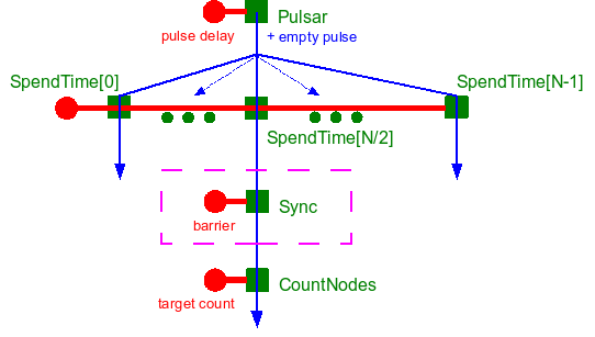
Figure 5: Conceptual system graph for example3
In example3, a pulsar sends empty pulses through a
user-defined number a concurrent cells, of custom
type CSpendTime that perform a meaningless computation of
random duration. A cell of custom type CCountNodes that
monitors the number of target nodes on the incoming active pulse is
connected downstream to one of the concurrent paths (the "middle" one
in this implementation).
The logical specifications for CSpendTime and CCountNodes are as follows:
| ex3::CSpendTime (fsf::CCell) | SPEND_TIME |
| Active filter | [FSF_ACTIVE_PULSE "Root"] |
| Passive filter | [FSF_PASSIVE_PULSE "Root"] |
| Output | (no output) |
| Performs a meaningless computation of random duration | |
| ex3::CCountNodes (fsf::CCell) | COUNT_NODES |
| Active filter | [FSF_ACTIVE_PULSE "Root" [FSF_NODE "*"]] |
| Passive filter | [FSF_INT32_NODE "Target"] |
| Output | (no output) |
Counts the number of nodes on the active pulse and prints out the
count to cout if the count is different from a the target
number specified on the passive pulse
| |
See
the Doxygen-generated reference
guide for detailed descriptions of
CSpendTime.
and
CCountNodes.
A barrier synchronization unit comprised of a CSync cell
connected to a repository that holds a CBarrier node sits
between the CCountNodes cell and its
upstream CSpendTime cell. When active, the
synchronization cell holds each active pulse until all the target
nodes specified in the barrier node (as a filter) are found in the
active pulse (i.e. filtering is successful), or until a timeout delay
has elapsed.
The logical specification for CSync is as follows:
| fsf::CSync (fsf::CCell) | FSF_SYNC |
| Active filter | [FSF_ACTIVE_PULSE "Root"] |
| Passive filter | [FSF_INT32_NODE "Barrier"] |
| Output | (no output) |
| Holds incoming active pulse until all the target nodes specified in the barrier node (as a filter) are found in the active pulse (i.e. filtering is successful), or until a timeout delay has elapsed | |
See
the Doxygen-generated mfsm
reference guide for detailed descriptions
of CSync
and CBarrier.
Without synchronization, the number of nodes on the active pulse depends on which paths is sampled. With barrier synchronization in before the monitoring, the number of nodes is always the same, equal to the total number of paths (except if the barrier times out on some of the paths).
The example implementation allows the user to specify on the
command line, among others, the pulse rate, the number of paths, and
whether to activate the barrier synchronization. Below are sample
outputs from the program without and with barrier
synchronization. Recall that the CCountNode cell prints
the number of nodes found in the active pulse when the number is
different from the number of concurrent paths.
Without synchronization (the sampled stream out of the requested 100 is the 50th):
example3 -f 30 -n 100 -s false
MFSM Example3: barrier synchronization
Alexandre R.J. Francois
(C) 2010
Requested pulse rate: 30 Hz
Number of // paths: 100 (not synchronized)
Starting cells...
53
51
50
53
50
53
50
50
53
50
50

Stopping the cells...
Cleaning-up...
Quitting program.
With synchronization (the sampled stream out of the requested 100 is the 50th):
example3 -f 30 -n 100 -s true
MFSM Example3: barrier synchronization
Alexandre R.J. Francois
(C) 2010
Requested pulse rate: 30 Hz
Number of // paths: 100 (synchronized)
Time out: 10 ms
Starting cells...

Stopping the cells...
Cleaning-up...
Quitting program.
references
Alexandre R.J. François, "An Architectural Framework for the Design, Analysis and Implementation of Interactive Systems," The Computer Journal, to appear.
Alexandre R.J. François, SAI: Architecting Distributed Asynchronous Software Systems, IMSC Technical Report IMSC-05-003, University of Southern California, Los Angeles, September 2005. [pdf] [BibRef]
Alexandre R.J. François, "A Hybrid Architectural Style for Distributed Parallel Processing of Generic Data Streams," Proceedings of the International Conference on Software Engineering, pp. 367-376, Edinburgh, Scotland, UK, May 2004. [pdf] [BibRef]